EMC Testing Part 2 – Conducted Emissions

EMC Testing Part 2 – Conducted Emissions

By Eur Ing Keith Armstrong C.Eng MIEE MIEEE, Partner, Cherry Clough Consultants,

Tim Williams C.Eng MIEE, Director, Elmac Services

Both Associates of EMC-UK

This is the second in a series of seven bi-monthly articles on ‘do-it-yourself’ electromagnetic compatibility (EMC) testing techniques for apparatus covered by the European EMC directive. This series will cover the whole range of test methods – from simple tests for development and fault-finding purposes, through lowest-cost EMC checks; ‘pre-compliance’ testing with various degrees of accuracy, on-site testing for large systems and installations; to full-specification compliance testing capable of meeting the requirements of national test accreditation bodies.

Of course, what is low-cost to an organisation of 5000 people could be thought fairly expensive by a company of 50, and might be too expensive for a one-person outfit, but we will cover the complete range of possible costs here so that no-one is left out. Remember though, that the more you want to save money on EMC testing, or reduce the likelihood of being found selling non-compliant products, the cleverer and more skilled you need to be. Low cost, low risk and low EMC skills do not go together.

This series does not cover management and legal issues (e.g. how much testing should one do to ensure compliance with the EMC Directive). Neither does it describe how to actually perform EMC tests in sufficient detail. Much more information is available from the test standards themselves and from the references provided at the end of these articles.

The topics which will be covered in these seven articles are:

1) Radiated emissions

2) Conducted emissions

3) Fast transient burst, surge, electrostatic discharge

4) Radiated immunity

5) Conducted immunity

6) Low frequency magnetic fields emissions and immunity; plus mains dips, dropouts, interruptions, sags, brownouts and swells

7) Emissions of mains harmonic currents, voltage fluctuations, flicker and inrush currents; and miscellaneous other tests

Table of contents for this Part

2 Conducted emissions

2.1Transducers for conducted emissions tests

2.1.1 Close-field probes

2.1.2 ‘Bug detectors’

2.1.3 Current probes

2.1.4 Absorbing clamps

2.1.5 Voltage probe

2.1.6 Errors in non-invasive measurements due to

impedance variations

2.1.7 LISNs and AMNs

2.1.8 Measuring CM and DM with LISNs

2.1.9 Transient limiters

2.1.10 ISNs

2.2Development, diagnostic, and QA testing

2.2.1 Using oscilloscopes

2.2.2 Using low-cost spectrum analysers

2.2.3 Using radio receivers

2.3‘Pre-compliance’ testing

2.4On-site testing of systems and installations

2.5Full compliance testing

2.5.1 Mains conducted tests

2.5.2 Telecom cables

2.5.3 ‘Disturbance power’ tests

2.6Discontinuous disturbances

2.7Instrumentation requirements for conducted and radiated

emissions tests

2 Conducted emissions

Part 0 of this series [1] described the various types of EMC test that might be carried out, including:

· Development testing and diagnostics (to save time and money)

· Pre-compliance testing (to save time and money)

· Full compliance testing

· QA testing (to ensure continuing compliance in volume manufacture)

· Testing of changes and variants (to ensure continuing compliance)

And Part 0 also described how to go about getting the best value when using a third-party test laboratory.

This part of the series focuses on testing conducted emissions to the typical domestic / commercial / industrial EN standard mainly over the frequency range 150kHz to 30MHz. There are many other kinds of conducted tests [2] and for other test standards some people will need to measure above 30MHz, and some people might need to measure below 150kHz. Military conducted emissions testing also covers a much wider frequency range than 150kHz to 30Hz.

Section 2.7 at the end of this article is a useful discussion of the characteristics of EMC emissions instrumentation of interest for both conducted and radiated testing.

Important Safety Note: When carrying out conducted emissions tests on mains or other electrically hazardous conductors, all appropriate safety precautions must be taken. These tests can be dangerous.

2.1 Transducers for conducted emissions tests

2.1.1 Close-field probes

Close-field magnetic and electric field probes are low-cost to buy and very quick and easy to make. They are commonly used in development, diagnostic and QA work. These transducers can easily be home-made, and were described in some detail in Part 1.1 of this series [1].

For conducted emissions at frequencies below 30MHz, larger diameter or multi-turn magnetic loop probes are preferred. Measuring conducted emissions is just the same technique as measuring radiated emissions with one of these probes: the probe is touched against the cable and oriented to obtain the maximum signal (usually when the plane of the coil is aligned with the cable run, with the cable at the furthest point of the probe. When testing product emissions, apply the probe close to the point where the cable concerned leaves the body of the equipment under test (EUT).

Close-field probes can be connected to oscilloscopes, EMC receivers, or spectrum analysers, and can be very useful in skilled hands as diagnostic or QA tools, especially if a ‘golden product’ is available for comparison as described in section 1.9 of Part 1 of this series [1].

Make sure all probes are insulated sufficiently to cope safely with the voltages being tested. Pin probes (see figure 2 of [1]) may be used on low-voltage signal conductors, but never on hazardous voltages such as mains. Use the special Voltage Probe (see 2.1.5 below) for all hazardous voltages.

2.1.2 ‘Bug detectors’

Part 1.3 of [1] described ‘bug detectors’ for identifying high levels of radiated emissions above 30MHz, but similar devices can be designed, and are commercially available, for detecting magnetic fields and may be used to indicate approximate levels of conducted emissions in development, diagnostic and QA testing.

To detect conducted emissions, these devices should usually have their insulated sensing tip touched against the cable being measured, close to the EUT. These probes are uncalibrated and neither are they frequency selective – they merely tell you by means of a meter or bar-graph whether there is a lot of emissions present or not. Some ‘bug detectors’ can identify the frequency of the strongest signal, and some provide outputs which can be connected to oscilloscopes, receivers, or spectrum analysers, enhancing their value considerably by allowing frequency discrimination, but of course their amplitude versus frequency response is almost always uncalibrated so they can’t be used to make measurements against test limits.

Despite their limitations, bug detectors can be very useful in skilled hands as diagnostic or QA tools, especially with a ‘golden product’ (see section 1.9 of [1]).

2.1.3 Current probes

These were described in Part 1.2 of this series [1], including how to make your own. Figure 1 shows some examples of commercially available clip-on probes, very handy for making quick comparison measurements. Because current probes can be calibrated they are also used for full compliance testing of conducted emissions to some military standards (not covered here) and an alternative method for measuring conducted emissions on telecommunication lines to the 1998 edition of EN 55022 (= CISPR 22:1997), see 2.5.2 below.

A different type of current probe is the Rogowski coil, basically a single-turn loop around the conductor whose current is to be measured. Their frequency response is not the highest, but they can be used to measure currents of thousands of Amps up to 1MHz, so can be very useful in power generation and heavy power applications where other transducers can’t cope. Figure 2 shows a commercially available product based on this technology.

In use, current probes are simply clipped over the cable to be measured, close to the EUT. Common-mode (CM) currents can easily be measured by clipping the probe over the entire cable so that both the send and return paths are included.

However, clipping a probe over just one conductor measures CM and Differential-Mode (DM) at the same time. To measure DM would require passing the send conductor through the probe in the opposite direction to the return, cancelling the CM signal and doubling the amplitude of the DM signal. Alternatively use two identical current probes, one on the send and one on the return conductor, and subtract their outputs using a transformer (broadly as described in section 2.1.8 below). Of course, trying to measure DM with a clip-on probe would disturb the arrangement of a cable and could cause errors at higher frequencies.

Current probe repeatability is enhanced at high frequencies by ensuring that the cables being measured are always positioned in the centre of the probe.

2.1.4 Absorbing clamps

The CISPR absorbing clamp has been used for many years for the disturbance power test of EN 55014-1 (CISPR 14-1), and to a lesser extent for certain apparatus in EN 55013 (CISPR 13). It is in essence a clip-on current probe (see earlier) combined with its own impedance stabilisation in the form of a series of plain clip-on ferrite rings. Figure 3 is taken from [3] and shows a variety of commercially-available absorbing clamps.

The plain ferrite rings absorb the RF power in the cable downstream of the measurement point. The limitations of ferrite mean that their impedance stabilisation becomes progressively less effective at lower frequencies, and this limits its use in full compliance testing to frequencies above 30MHz. However it is a convenient and non-invasive way to couple to a cable and this makes it attractive for many purposes. Like all magnetic field probes and current clamps it measures only the magnetic field surrounding the cable and so does not need a ground reference plane.

Clearly, those with a flair for working in wood or plastic can easily make their own absorbing clamp. A useful guide to the features and use of absorbing clamps can be found in [3].

2.1.5 Voltage probe

CISPR, ANSI, and the FCC all describe a voltage probe which can be used to measure the conducted emissions on power terminals, usually when LISNs (see below) aren’t available or aren’t appropriate, often due to the high currents involved. Figure 4 shows the basic schematic for a voltage probe, plus an example of a commercially available model.

Safety Note: To help prevent damage to the measuring equipment the capacitor should be a class Y type, and to prevent electric shock the probe and its output should be suitably insulated and designed with a handle that keeps its user’s fingers protected from the terminal being probed.

2.1.6 Errors in non-invasive measurements due to impedance variations

The close-field probes, ‘bug detectors’ current probes, absorbing clamps or the voltage probe described above are non-invasive and do not require the conductor being measured to be interrupted. Consequently they are easy and quick to use. Unfortunately, where the CM and/or DM impedances of the measured circuit are not controlled during testing the emissions measured for a given EUT can depend on its installation.

Despite this, some test standards allow such tests in certain situations, presumably because they are better than no tests at all. However, most of the conducted emissions tests in standards harmonised under the EMC directive require impedance control to give repeatability, and below 30MHz this usually means an invasive test method using LISNs or ISNs, as described in 2.1.7 and 2.1.10 below.

Measurements with current probes, absorbing clamps and voltage probes can be made repeatable if the impedances of the conductors are stabilised by using LISNS or ISNs which have their RF outputs terminated in 50W. Some standards accept current probe results when tests are set up in this way.

But even with impedance stabilisation of conductors the results from close-field probes and ‘bug detectors’ are always going to be non-repeatable to some degree – if only because they are usually very sensitive to position and orientation and it is difficult to hold them exactly the same way twice.

2.1.7 LISNs and AMNs

Line Impedance Stabilisation Networks (LISNs) – sometimes called Artificial Mains Networks (AMNs) are the standard transducer for measuring conducted emissions in a great many test standards. They are invasive transducers which must be connected in series with the conductors being tested to standardise their CM and DM impedances. Reference [3] is a detailed analysis of LISNs and their application. Figure 5, which is taken from [3], shows five commercially available LISNs.

A LISN couples the interference from the EUT connection to the measuring equipment and at the same time presents a stable and well-defined impedance to the EUT across the desired frequency range. The actual measured voltage depends on the ratio of the EUT’s source impedance and the LISN’s load impedance, so if the impedance were not stabilised, there would be no repeatability between different test locations. CISPR defines the LISN and its impedance for some different classes of network: the most common one is shown in Figure 6 and is known as the “50Ohms/50µH+5Ohms” network, since the impedance curve is determined by these values.

Figure 7 shows that its frequency response is defined down to 9kHz and a fully compliant LISN will stay within the specified tolerance of ±20% of this curve whatever the termination at the mains side of the unit. This is easily achieved across most of the frequency range, but poorly designed units can exceed the specification below 50kHz or above 25MHz. Figure 7 also shows the impedance curve for a different type of LISN, a “50W/5µH+5W” network which is sometimes specified where currents are very high.

The 1kW resistors shown in Figure 6 are there to discharge the 0.25mF voltage coupling capacitors when no external termination is fitted, helping to prevent damage to sensitive RF ‘front ends’. The use of transient limiters (see 2.1.9) should protect against such damage, but 1kW resistors are cheap and the RF front ends expensive so why take the risk.

Like all EMC transducers, LISNs must be calibrated and their calibration factors (sometimes called transducer factors) taken into account whenever they are used in an accurate measurement of conducted emissions.

The LISN’s earth is connected to the ground reference plane (GRP) of the test setup. Since this is the ground reference for the measurement, no extra RF impedance should be introduced by this connection because it would affect both the impedance seen by the EUT and the voltage developed across the LISN’s impedance. This means that wires or straps of more than a few inches must not be used, since their inductance is unacceptable. The best connection here is a solid metal bracket, firmly bonding the LISN to the GRP, as shown by Figure 8 (taken from [3]).

Perfectly good LISNs can be purchased for around £600 (UK Pounds), but if you wish to construct your own you should recognise that constructing an accurate LISN is not as simple as its schematic. Here are a few essential construction tips extracted from [3] and [4]:

· For the 50mH inductor, follow the construction shown in Figure 9 (taken from [4]) an example of which is given in Figure 10.

· Use a number of large-value safety-rated capacitors (preferably Y1 rated) in parallel for the 8mF parts, and low-inductance resistors (not wire-wound types) for the 5W. Keep all lead lengths very short and use the chassis of the unit as the earth connection for the schematic, rather than any earth wires. Any unavoidable wired earth connections (e.g. from the earth pin of the EUT mains socket to the chassis must be no longer than 50mm and should use braid straps or metal plates at least 10mm wide.

· For the general assembly of the LISN follow the sketch of Figure 11 (taken from [3]).

Ferrite-cored inductors are available (for example from Newport Components) which are much smaller than the air-cored components described above and permit the construction of very compact LISNs. When using a ferrite-cored inductor for a LISN, bear in mind that most AC-DC mains input equipment power supplies do not draw sine-wave currents and if the size of the core is inadequate it may saturate at the current peaks and give incorrect results.

Commercially available LISNs may be fitted with ‘added value’ enhancements to the circuit of Figure 6, such as additional low-pass filtering for the incoming mains, and high-pass filtering for the RF output to remove most of the mains frequency.

LISNs create an artificial supply impedance of 50W from each line to earth making the common-mode (CM) impedance 50W and the differential-mode (DM) impedance 100W, both across a wide range of frequencies, whereas real mains supplies have CM and DM impedances that vary from 2W to 2000W (at least) depending upon the mode, the time of day, and the frequency (above 10kHz).

This means that filters which give good results on a conducted emissions test might not provide the same degree of filtering in real applications. For more on the problems of source and load impedances for filters, and on how to choose filters which do give reliable filtering both on LISN tests and for a very wide variety of real-life impedances, refer to section 3.8 of [5], or section 8.1.3.1 of [6].

A Very Important Safety Note for All LISNs and AMNs

Because of the lethally-high earth-leakage currents created by the 8mF capacitors, all LISNs must have two independent protective earth connections in place before the mains voltage is applied to them. Each protective earth connection must be rated for the full value of the possible fault current (i.e. the maximum current if the live supply should short-circuit directly to the chassis).

Staff training in the safe and correct use of LISNs is strongly recommended, and untrained people and third parties must not be allowed to be within reach of LISNs or equipment or cables connected to them. A regular and documented safety check of the integrity of both the protective earth bonds is also recommended.

Warning labels on LISNs are also strongly recommended for:

· their lethally high earth-leakage current

· the need to maintain two independent protective earth connections at all times

· their use only by authorised and trained personnel

If your purchased (or home-made) LISN does not have the necessary warning labels already fitted, add them immediately – in very conspicuous places.

Because of the high levels of continuous earth-leakage currents associated with LISNs and AMNs, residual current circuit breakers (RCCBs) and other types of earth-leakage protection devices can’t be used.

2.1.8 Measuring CM and DM with LISNs

The RF outputs from a LISN are neither CM or DM, they are a mixture of the two. But it helps to know whether emissions are CM or DM when designing or selecting filters. CM can be measured by summing all the LISN’s RF outputs together, and DM by the difference between the RF outputs.

It is relatively easy to obtain CM and DM from a single-phase LISN using a multi-channel oscilloscope, but the results will be in the time domain unless the ‘scope has FFT to convert them to frequency domain. Unfortunately most RF measuring instruments can’t do sum and difference like a ‘scope can, but a simple transformer wound on a ferrite toroid or pot core can provide the necessary outputs, as shown by Figure 12 which has been taken from [7].

2.1.9 Transient limiters

These aren’t transducers, but nevertheless need calibrating. They fit between the LISN and the measuring instrument to protect the instrument from mains transients. The LISN itself will attenuate most of the transients on the mains supply – the real problem is the connection and disconnection of the EUT, which can cause 400V transients to appear at the RF outputs.

Limiters usually consist of a -10dB attenuator plus a pair of back-to-back small-signal diodes to clip the maximum signal to about ±1V. They should be calibrated, and their ‘correction factors’ taken into account along with the LISN’s own transducer factors and any correction factors for the cables, on every measurement where they are used.

(Some EMC receivers or spectrum analysers have built-in transient limiters, in which case they are calibrated when the test instrument is calibrated and can be ignored.)

2.1.10 ISNs

Impedance Stabilising Networks (ISNs) are often broadly similar in design and construction to LISNs and are used to make conducted emissions measurements on signal and data cables. Like LISNs, they are invasive transducers which must be connected in series with the conductors to be measured to standardise their CM and DM impedances. ISNs differ from LISNs in that they are designed to measure CM conducted emissions. Also, whereas LISNs create an impedance of 50W, ISNs create an impedance of 150W because this is thought to more closely match the real impedances of signal and data cables.

Figure 13 shows an example of an ISN taken from the 1998 issue of EN 55022. This ISN design is very similar to the coupling-decoupling networks (CDNs) specified by the conducted immunity test IEC 61000-4-6, and in fact it may be possible to use these CDNs as ISNs in some cases. Several other types of ISNs are specified in this standard, not all of which use a similar circuit.

2.2 Development, diagnostic, and QA testing

2.2.1 Using oscilloscopes

Please refer to section 1.5 of Part 1 of this series [1] for a detailed discussion of using ‘scopes and their voltage probes for some types of EMC testing. For conducted emissions the frequency response of the vertical channels of the ‘scopes used and any probes need only be 50MHz, so low-cost instruments can be used.

All the transducers described above can be connected to oscilloscopes if a 50W termination is applied at the ‘scope input (either by selecting the 50W termination option, or by fitting an external 50W termination). Standard high-impedance voltage probes can also be connected to signal and data conductors (not mains! – see below) to measure their CM or DM voltage noise, although this will usually vary depending on the CM and DM impedances of the installation or test set-up – making comparisons difficult unless an ISN (see above) is also used or the impedances are fixed in some other way.

For a CM measurement all the conductors in a signal or data cable (including their signal returns) should be probed and their channels summed in-phase (A+B). For a DM measurement each conductor should be probed and their two channels subtracted (A-B). The ground leads for the ‘scope probes should not be connected to anything (neither any of the conductors being tested or the EUT chassis) and as a result CM measurements will tend to suffer from high levels of mains frequency. This can be reduced by using high-pass filters with good rejection at mains frequency and no attenuation for the frequencies to be measured. Some ferrite chokes on the probe leads, or on the mains lead to the ‘scope, can help reduce high-frequency CM interference and is described in more detail in 1.5 of [1].

When connecting a ‘scope to a LISN or ISN RF output or to a mains voltage probe high levels of mains-frequency can once again be a problem, and the high-pass filter mentioned above can be very useful.

Using ’scopes and probes is clearly the lowest-cost way to do development or diagnostic emissions testing, but requires quite a lot of skill in reading waveforms to achieve any quantitative correlation with standard EMC tests. ‘Golden product’ testing, described in detail in section 1.9 of [1] is recommended as a means of learning what correlations may reasonably be made.

So with a small outlay (or none), a bit of a learning curve, and a ‘golden product’, a typical electronic designer can obtain useful EMC information by simply using a ’scope, plus (ideally) LISNs, ISNs, or other suitable conducted emissions transducers.

Safety Notes for ‘scopes: Remember – equipment safety earths must NEVER be removed. If you have a ‘ground loop’ problem, deal with it by using ferrite CM chokes, isolating transformers, differential amplifiers, or whatever, but never remove a protective earth lead from any equipment or EUTs.

Also remember that normal ‘scope probes are not rated for mains use and are probably not safe when used in this way. The Voltage Probe described in 2.1.5 above (preferably purchased 3^rd-party approved to EN 61010) should be used instead.

’Scope probe ground leads should never be connected to mains neutral. Although the neutral is connected to earth at some point in the distribution network, voltage drops due to heavy currents flowing along the length of the neutral, plus 3-f imbalances, can mean that the neutral has a few volts on it sourced from under 1W, capable of driving a few amps through the probe ground and the ‘scope, and possibly causing some damage. (Up to 60V has been seen on the neutral in some buildings, making a probe’s ground lead start to smoke within seconds.)

2.2.2 Using low-cost spectrum analysers

Spectrum analysers are ideal tools for development, diagnostic, and QA testing of conducted emissions, and electronic hardware design and development can benefit hugely from being able to see the frequency domain being used. Please refer to section 1.6 of Part 1 of this series [1] for a detailed discussion of spectrum analysers, including low-cost types and second-hand models, problems with their detectors, how to avoid input overloads that can give erroneous readings, plus the use of ‘golden product’ testing to improve their usefulness.

Spectrum analysers can be used with close-field probes, current probes, absorbing clamps, voltage probes, LISNs and ISNs. The typical ’scope probe could also be used (on non-hazardous voltages only) but beware of the effects of the spectrum analyser’s 50W input impedance and susceptibility to damage. Whenever making a direct voltage measurement with a spectrum analyser, be very careful to attenuate any DC or low-frequency signals so they don’t burn out its very sensitive (and expensive to replace) input devices.

2.2.3 Using radio receivers

Here we are considering the use of the ‘canteen radio’ and similar everyday radio receiver products for EMC diagnostics and QA work. Please refer to section 1.7 of Part 1 of this series [1] for a detailed discussion of their advantages (low-cost) and how to overcome their many disadvantages when using them for EMC testing.

Using radios to test for conducted emissions is much the same as using them to test for radiated emissions (see 1.10 of [1]) – except that the frequency range is different. Most commercial and industrial emissions standards under the EMC directive require testing conducted emissions down to 150kHz, which is the bottom of the long-wave band on most AM radios.

Most domestic radio receivers use a ferrite rod antenna for the long and medium wave bands (up to 1MHz), and this may require a different set-up to tests done at higher frequencies using a telescopic antenna. For example, one of the authors, working on a phase-angle-controlled power controller recently, found that when the EUT’s mains cable was wrapped twice around the body of a portable AM radio, and it was tuned between the stations on the LW and MW bands with the volume control set to a set level, the level of audible ‘buzz’ correlated very well with results on an accredited conducted emissions test for the type of EUT concerned. (This test method could have been improved by measuring the RMS value of the audio output by connecting a true-RMS voltmeter to the radio’s headphone output, and plotting graphs of amplitude against the radio’s tuner frequency.)

2.3 ‘Pre-compliance’ testing

General issues of pre-compliance emissions testing were covered in section 1.8 of Part 1 of this series [1] as they applied to radiated emissions testing. The same general conclusions can be drawn for conducted emissions testing – follow the full test method as closely as you can, and calculate (or at least estimate) your measurement errors and take them into account.

Conducted emissions testing is relatively easy to do with high accuracy in the comfort of your own building. The site requirements are very relaxed compared with the problems of radiated testing, and a simple arrangement of metal plates can be sufficient if the ambient is quite enough. Where noisy ambients are a problem (either conducted on the mains supply or radiated) a low-cost shielded room with filtered mains can be used, such as those shown in Figures 14 and 15. There is no need for absorber in the room.

The full testing method is described below and should be followed as far as is needed for the accuracy required when pre-compliance testing. More detailed advice on pre-compliance conducted measurements using a spectrum analyser can be found in [8].

2.4 On-site testing of systems and installations

This was discussed in general, and from the point of view of radiated emissions testing, in section 1.11 of Part 1 of this series [1]. Chapter 10 of [6] is also a useful reference.

Which ground reference to use is a crucial factor when testing on-site. In test laboratories it is defined by the ground reference plane (GRP) but in-situ referencing has to make do with what exists and what can practically be achieved. CISPR 16-2 recommends the following:

The existing ground at the place of installation should be used as reference ground. This should be selected by taking high frequency (RF) criteria into consideration. Generally, this is accomplished by connecting the EUT via wide straps, with a length-to-width ratio not exceeding 3, to structural conductive parts of buildings that are connected to earth ground. These include metallic water pipes, central heating pipes, lightning wires to earth ground, concrete reinforcing steel and steel beams.

In general, the safety and neutral conductors of the power installation are not suitable as reference ground as these may carry extraneous disturbance voltages and can have undefined RF impedances.

If no suitable reference ground is available in the surroundings of the test object or at the place of measurement, sufficiently large conductive structures such as metal foils, metal sheets or wire meshes set up in the proximity can be used as reference ground for measurement.

“Sufficiently large” probably means that the added metal foils, sheets, or meshes should underlie the whole of the EUT and spread beyond it for at least half its height, so as to maximise its stray capacitance. But it all depends on what you are trying to achieve – if you are trying to test a product which will be manufactured in volume and sold into other environments, maximising stray capacitance with metal sheets corresponds more closely to the proper test set-up (see 2.5 below) and represents a worst-case set-up.

However, if you are measuring the conducted emissions from a custom-made item of apparatus when it is installed at the site where it is permanently installed, to determine whether this single apparatus is compliant as installed (for example when following the Technical Construction File route for the compliance of a large system) then it is more reasonable to use only the existing bonded metal structures and not add to them.

Both LISN and voltage probe tests require a reference, which would typically be the boundary of the system where the power supply connects to it, often the terminals of a power outlet or a supply transformer dedicated to the system. Transducer reference connections must be bonded using a short, wide strap to the chosen reference point – lengths of green-and-yellow wire are not adequate.

The layout of the mains cable should be as close as possible to normal operation during the test and excess cable or coils of cable should be avoided. Whatever the mains cable layout is, it should be fixed for the duration of the tests and drawn (or photographed) for the test report.

Almost no test standards provide adequate guidance for in-situ testing, so site-specific test plans have to be developed. Many decisions will have to be taken by EMC engineers on the spot. Some basic practices which apply to conducted tests in the laboratory also apply here:

· Take an ambient scan with the EUT switched off. Create a list of ambients.

· With the EUT switched on and operating, take a peak detector sweep with a reasonably fast scan speed, taking into account the EUT’s cycle time, to create a list of significant emission frequencies. Subtract known ambients from this list, leaving a list of ‘suspects’.

· Test the suspect frequencies individually using the quasi-peak and average detectors as required to make the comparison with the limits in the relevant standard, modifying the EUT’s operation to maximise the emissions if this is relevant.

· It is a good idea to recheck the ambients from time-to-time during a test to make sure that new ambient sources (such as someone using an electric drill nearby) aren’t being mistaken for EUT emissions.

This procedure is repeated for all the mains phases at each location to be measured.

2.5 Full compliance testing

Virtually all CISPR-based test standards specify limits on conducted emissions measured from 150kHz to 30MHz at the mains port. The three most commonly referenced standards EN 55011, 55014-1, 55022 (CISPR 11, 14-1 and 22 respectively) all set such limits and their methods are largely common, although there are detailed differences. EN 55013 and 55015 (CISPR 13 and 15) for broadcast receivers and lighting equipment respectively also require a similar test, although EN55015 extends the measurement down to 9kHz for some apparatus.

Two other more specialised conducted test methods are significant: the absorbing clamp method of CISPR 13 and 14-1 and the new telecom port test of CISPR 22.

2.5.1 Mains conducted tests

To appreciate the constraints on fully compliant conducted tests you have to be familiar with the test equivalent circuit (Figure 16). This shows that in the mains port test you are measuring a combination of DM and CM sources on each line (L or N) with respect to the ground reference plane (GRP), which is connected to the EUT’s ‘earth’ connections if it has any.

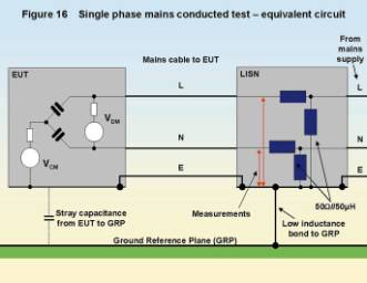
The factors outside the EUT that control the coupling, and hence the measured value, are:

· Stray capacitance from EUT to GRP

· RF impedance of the mains cable

· RF impedance of the LISN

The equivalent circuit shows that stray capacitance between the EUT and the GRP is an important part of the coupling path. The standard test set-up for table-top EUTs is shown by Figure 17 (similar to figures 7 and 9 in EN 55022:1998) and regularises stray capacitance by insisting on a fixed separation distance between the two; 400mm is the norm, with at least 800mm clearance from all other conducting surfaces. For a fully compliant test you should be scrupulous in observing these distances. All test houses have an 800mm wooden table on which the EUT can be sideways spaced by 400mm from a vertical GRP. An alternative that is allowed in some standards is a 400mm separation from the bottom of the EUT to a horizontal GRP.

The third important aspect is the impedance introduced by the mains cable. This is not negligible above 15-20MHz and it must be controlled. Laying it on the GRP will introduce excess stray capacitance; coiling extra length will introduce more inductance. Keeping it off the GRP, and bundling it if necessary in the way prescribed by the standard, controls both these factors and minimises the variations introduced by the cable. Bundling is still somewhat hit-and-miss and it is a good idea to use a standard unbundled 1m length of cable for your tests, whatever length the final product will be supplied with.

Figure 17 is only appropriate for table-top EUTs, and all the necessary set-up details for these and other styles of EUT (e.g. floor standing equipment) will be found in the relevant sections of the appropriate test standard. Reference [9] contains some useful detail on performing full compliance conducted emissions tests, especially as regards the control of the test instrumentation.

2.5.2 Telecom cables

CISPR 22 third edition now includes a new suite of conducted emissions tests on ports intended for connection to telecom networks, particularly PSTN or LAN connections. More work still needs to be done to clarify the test methods, which are in some cases difficult to implement; the EMCTLA have recently published Technical Guidance Note TGN 42 and its Addendum 1 [10] gives additional interim guidance to test houses, especially valuable at this time because there has been a series of errors which means that many ISNs are 10dB in error at the time of writing.

Essentially, the preferred method is to use an Impedance Stabilising Network (ISN) transducer as described in section 2.1.10 above. This couples the CM signal off the cable under test while ensuring a fixed CM impedance to the GRP, in this case 150W, over the measured frequency range. The difficulty occurs with cables which carry wideband data, where the data signal is in the same frequency range as the interference measurement. In this case the ISN must not compromise the wanted DM signal transmission, and it must have a specified conversion between DM and CM which accurately reflects the longitudinal conversion loss of real cables. This has been a matter for some controversy.

A further difficulty occurs with cables for which no ISN is available, in which case an alternative method is given using both current and voltage measurements, since the CM impedance cannot be properly stabilised. This method is also controversial and can be difficult and cumbersome to carry out.

Having said this, some products are being successfully tested against these requirements. The factors to bear in mind are essentially the same as for the mains emissions tests – separation distances, cable layout, and proper bonding and calibration of the ISN. The example set-up in Figure 17 includes an ISN, and all the necessary set-up details will be found in the relevant sections of EN 55022:1998 (CISPR 22:1997).

2.5.3 ‘Disturbance power’ tests

Absorbing clamp transducers were described in 2.1.4 above, and are used by EN 55014-1 (CISRP 14-1) to measure ‘disturbance power’ over the frequency range 30 to 300MHz. This is a conducted emissions test being used where most other standards would use a radiated test, the assumption in the standard being that all the radiated emissions from an EUT are emitted from the cables attached to it. Poor correlation is found when comparing products fully tested using both the ‘disturbance power’ method and the OATS method described in section 1.12 of [1], but with experience and careful use of ‘golden products’ (see section 1.9 of [1]) it is often possible to use absorbing clamp tests as pre-compliance radiated emissions tests.

For pre-compliance use the absorbing clamp can be used at a fixed position on a cable (generally very close to the EUT) while comparison measurements are taken. But a full compliance test must take into account the standing waves that still exist on the cable even though the clamp has some absorbing effect. This means that the clamp must be moved through a half-wavelength along the cable from the EUT while searching for a maximum at each frequency. Half a wavelength at 30MHz is 5m, and therefore a “raceway” is used along which the cable is stretched, so that the clamp can be rolled along it during the measurement.

EN 55014-1 is quite relaxed about the test set-up, and a fully compliant test can be performed in virtually any environment and with the cable terminated in virtually any way. Recent work to quantify the uncertainties of the method has shown that it is best to terminate the far end of the cable with a second clamp or a string of clip-on ferrites, to keep conductive objects (including people) well away from the cable under test, and to ensure that the cable passes through the centre of the clamp aperture.

2.6 Discontinuous disturbances

The final test to be discussed here is the discontinuous disturbances test of EN 55014-1 (CISPR 14-1), which is usually applied to automatically operating electro-mechanical circuit breakers such as the bi-metal strip ‘energy regulators’ in cooker hotplates and ovens, and the automatic control of heaters, pumps, or motors in a variety of applications.

According to the standard, the EUT is set-up exactly as for a normal conducted emissions test on the mains cable, but the IF output of a receiver or spectrum analyser is viewed using an oscilloscope with the receiver or analyser set to measure a few specified frequencies between 150kHz and 30MHz. Sometimes it is possible to omit the receiver or spectrum analyser and connect the ‘scope directly to the output of the LISN (usually via a high-pass filter to remove the mains frequency and also via an attenuator because of the high voltages which can occur).

Various characteristics of the duration and repeat rate of the transients observed on the ‘scope (an analogue storage ‘scope is recommended) are noted and compared with a complex set of tables and instructions to decide whether the transients are compliant. Generally speaking, if all the transients observed last for less than 10ms, and don’t occur more than 5 times a minute on average, they are compliant with the limits in this part of the standard regardless of their amplitude.

Watching the transients on the ‘scope screen and comparing them with the very arcane rules in the standard is not most EMC engineers’ idea of a pleasant time. It is quite easy to design and make simple equipment to give a go/no-go indication suitable for QA testing for discontinuous emissions, and rather more difficult to make an instrument suitable for automatic pre-compliance testing. There are very few instruments designed for automatic compliance testing of discontinuous disturbances, such as Figure 18.

2.7 Instrumentation requirements for conducted and radiated emissions tests

Interference measuring receivers have to comply with the provisions of CISPR 16-1 if they are to be used for full compliance measurements. Much has been written about the merits of “pre-compliance” equipment, which is, of course, cheaper. To understand the issues it is worth a brief look at the constraints imposed by the specifications of CISPR 16-1. These are, in no particular order:

· Bandwidth

· Detectors

· Overload performance and pulse accuracy

· Input VSWR and sensitivity

– and they are equally applicable to the radiated measurements described in Part 1 of this series [1] as they are to the conducted tests being described in this part.

If an interference signal spectrum is wider than the bandwidth of the instrument which measures it, then the indicated value will depend on that bandwidth. If it is narrower, then the indicated value is independent of bandwidth. This is the basis of the distinction between “narrowband” and “broadband” interference. If you are measuring known radio signals then you can tailor the measurement bandwidth to the characteristics of the signal, but this is not possible for EMC measurements, since the characteristic of the interference is almost by definition not known in advance. Therefore the measuring receiver specification must include a defined value not only for the bandwidth, but for the shape of the filter that determines this bandwidth. This specification is given in Figure 19.

Only a receiver whose bandwidth characteristics fully comply with this specification should be used for full compliance measurements. However, if you are only measuring narrowband interference, such as individual emissions from the harmonics of microprocessor clocks, the actual performance of the receiver filters will have little or no effect on the outcome. This is the root of much of the confusion over bandwidth requirements.

CISPR 16-1 specifies three principal detector types, peak, quasi-peak and average. Most initial measurements are made with the peak detector, which as its name implies responds almost instantly to the peak value of the interference signal seen at its input. Radiated emissions limits are specified by standards using the quasi-peak detector (although some recent ETSI standards use the peak detector). Conducted emissions limits are specified for both the quasi-peak and average detectors. Full compliance measurements must use only the correct detectors. The difference between the detectors resides in how they respond to pulsed or modulated signals, as shown in Figure 20. All three types of detector give the same response to unmodulated, continuous signals.

The quasi-peak detector weights the indicated value in terms of its perceived “annoyance factor”: low pulse repetition frequencies (PRF) are less annoying when experienced on broadcast radio and TV channels than high PRFs. The detector is specified in terms of its attack and decay time constants, and these are fairly straightforward to implement. The average detector simply returns the average value rather than the peak value of the interference with which it is presented. This can in principle be achieved with a simple low-pass filter whose time constant is slower than the slowest pulse repetition frequency of the input.

The difficulty which faces designers of measuring receivers is that to give an accurate measure of the actual quasi-peak or average level of low PRF interference, the linear dynamic range of the RF circuits before the detector, and of the detector itself, must be at least equal to the dynamic range of the desired pulse weighting if the pulses are not to be compressed. This dynamic range according to the CISPR 16 specification can approach 43dB, which means closer to 60dB in the receiver design. If the receiver does not adjust its gain continually to achieve the optimum level at the detector – spectrum analysers, for instance, can’t do this – then the needed dynamic range is several tens of dB more. This is a serious design challenge for RF circuits, and as a result linearity and overload performance for pulsed signals are the most important factors which distinguish low-cost instruments from fully compliant measuring receivers.

Of somewhat lesser importance, but still part of the CISPR 16-1 spec, is the requirement on input VSWR (Voltage Standing Wave Ratio). This is specified to be 2:1 with no input attenuation, dropping to 1.2:1 with 10dB attenuation. VSWR is directly related to measurement error due to mismatch. For a broad spectrum receiver (remember, 9kHz to 30MHz is more than three decades) the spec of 2:1 without attenuation is quite hard to meet – many ordinary radio receivers can’t achieve this even over a narrow range. It’s easy enough if you allow yourself some attenuation at the input, but then the receiver sensitivity is degraded. The sensitivity requirement in CISPR 16-1 is expressed in the form that the noise component should not degrade the measurement accuracy by more than 1dB, which implies that the system noise floor must be at least 6dB below the lowest level it is desired to measure accurately. The system noise floor is the receiver noise plus the losses imposed by the transducer or antenna factor and connecting cables. In practice, the limiting performance is usually found at the top end of the radiated test around 1GHz. Low-cost receivers and antennas are often found to have inadequate sensitivity at these frequencies even to measure at the limit line, let alone below it.

In summary, there are several reasons for the high price of fully compliant measuring receivers, and the stringency of the CISPR specification is a direct result of the need to make accurate measurements, of an unknown and variable interfering signal, over an extremely wide range of the spectrum. Any “pre-compliance” instrument will necessarily compromise some or all of these aims.

References

[1] “EMC Testing Part 1 – Radiated Emissions” Keith Armstrong and Tim Williams, EMC + Compliance Journal February 2001, pages 27-39, can be read and downloaded from www.emc-journal.co.uk. (Also includes Part 0.)

[2] “The measurement of emissions (methods and instrumentation)” R. W. Gubisch, Compliance Engineering European Edition, January/February 1998, Pages 46-55, (part 2 of a series of 7 articles on EMC testing).

[3] “Calibration and use of artificial mains networks and absorbing clamps (Application of transducers for CISPR-based emissions measurements)” Tim Williams and Geoff Orford, DTI-NMSPU Project FF2.6 report, April 1999. May be available from the EMCTLA – see [10] below.

[4] “Proposed new CSA standard C108.1.5, Line Impedance Stabilising Network (LISN)” Canadian Standards Authority (CSA), C108.1.5, 4th draft, June 1984

[5] “Design techniques for EMC – Part 3: Filters and surge protection devices” Keith Armstrong, the UK EMC Journal, June 1999, pages 9-15, can be read and downloaded from www.emc-journal.co.uk.

[6] “EMC for systems and installations” Tim Williams and Keith Armstrong, Newnes, January 2000, ISBN 0-7506-4167-3 (available from RS and Farnell).

[7] “An alternate, complementary method for characterising EMI filters” Michel Mardiguian and Joel Raimbourg, IEEE EMC Symposium, Seattle 1999, Volume 2, pages 882-886.

[8] “Cookbook for EMC pre-compliance measurements” Application Note 1290-1, Agilent Technologies (previously Hewlett Packard)

[9] “Making radiated and conducted compliance measurements with EMI receivers” Application Note 1302, Agilent Technologies (previously Hewlett Packard)

[10] “EMCTLA Technical Guidance Note #42 – Emissions tests on telecom ports as per CIPSR22 (EN 55022)” plus its “Addendum 1”, Tim Williams, EMC Test Labs Association, P.O. Box 129, Romsey, SO51 6ZT, UK, www.emctla.org.uk

Corrections to Part 1

A number of commercial products were shown unattributed in the figures of Part 1 of the series. We apologise for this oversight, thank the suppliers of the photographs, and list them here:

Figure 3: a close field probe set from Laplace Instruments Ltd.

Figure 6: two types of ‘bug detectors’ from Laplace Instruments Ltd.

Figure 7: a very small antenna from York EMC Ltd.

Figure 10a: an OATS at York EMC.

Figure 10b: an OATS at EMC Technologies PTY Ltd of Melbourne Australia.

Figure 11: a shielding tent from Cornwell EMC (now Europatech Ltd).

Figure 12: a large semi-anechoic room at SEQAL, Yateley, Hants.

Figure 13: a large stirred-mode chamber at DERA, Farnborough, Hants.

Figure 14 and others: the ‘Bilog’ antennas are from York EMC Ltd.

Eur Ing Keith Armstrong C.Eng MIEE MIEEE
Partner, Cherry Clough Consultants, www.cherryclough.com, Associate of EMC-UK
Phone: 01457 871 605, Fax: 01457 820 145,

Email: keith.armstrong@cherryclough.com

Tim Williams C.Eng MIEE
Director, Elmac Services, www.elmac.co.uk, Associate of EMC-UK
Phone: 01243 533 361, Fax: 01243 790 535,

Email: elmactimw@cix.compulink.co.uk